monecascale: hierarchical DC-SBM backend for MONECA

About monecascale

monecascale is a sibling package to moneca. It provides scalable clustering backends whose output is consumed unchanged by moneca’s analysis and plotting stack. The first backend, moneca_sbm(), replaces moneca’s clique-enumeration step with hierarchical degree-corrected stochastic block model (DC-SBM) inference — the natural statistical twin of moneca’s relative-risk framing.

This vignette motivates the design, shows a minimal end-to-end workflow, reproduces the empirical parity measurement against moneca::moneca_fast(), and explains when to reach for which backend.

The theoretical bridge: RR = O/E is the DC-SBM residual

MONECA’s weight matrix is the relative-risk deviation of observed mobility from the independence null:

$RR_{ij} = \frac{O_{ij}}{\bigl(r_i \cdot c_j\bigr) / T}.$

The degree-corrected stochastic block model (Karrer & Newman, 2011) models the expected number of edges between nodes i and j as \theta_i \theta_j \omega_{g_i, g_j}, with \theta degree parameters and \omega a block-interaction matrix. Setting \omega to the identity yields exactly (r_i c_j) / T as the expected count — i.e., MONECA’s independence null. In that sense MONECA’s RR is the DC-SBM residual, and the clique rule on the thresholded RR is a hand-rolled approximation to block inference. Any modern DC-SBM inference routine is therefore a principled scalable drop-in.

Two backends are wired up behind moneca_sbm():

"greed" (default, R-native via greed::DcSbm): hierarchical dendrogram, Poisson likelihood for counts, sparse dgCMatrix input end-to-end, portable parallel via the future framework. Scales comfortably to ~10^4 – 10^5 nodes.
"graphtool" (opt-in, Python via reticulate): Peixoto’s minimize_nested_blockmodel_dl(), which uses merge-split MCMC to minimize description length directly. Scales to 10^6+ nodes on commodity hardware.

Quick start

library(monecascale)
library(moneca)

mob <- generate_mobility_data(
  n_classes = 20,
  n_total = 5000,
  immobility_strength = 0.5,
  class_clustering = 0.75,
  noise_level = 0.05,
  seed = 2026
)

seg <- moneca_sbm(mob, backend = "greed", seed = 2026)
seg
#> 
#> ================================================================================
#>                         moneca MOBILITY ANALYSIS RESULTS                        
#> ================================================================================
#> 
#> OVERALL MOBILITY PATTERNS
#> -------------------------------------------------------------------------------
#> Overall Population Mobility Rate:                    67.1%
#> Average Mobility Concentration (all levels):         94.8%
#> 
#> HIERARCHICAL SEGMENTATION ANALYSIS
#> -------------------------------------------------------------------------------
#> 
#> Internal Mobility Within Segments (%):
#>  Level 1  Level 2  Level 3  Level 4  Level 5  Level 6  Level 7  Level 8 
#>     32.9     42.9     44.0     46.6     47.5     49.2     52.8     54.1 
#>  Level 9 Level 10 Level 11 Level 12 Level 13 Level 14 Level 15 Level 16 
#>     55.6     60.9     69.9     75.0     78.0     86.1     90.9     92.7 
#> Level 17 
#>     95.8 
#> 
#> Mobility Concentration in Significant Pathways by Level (%):
#>  Level 1  Level 2  Level 3  Level 4  Level 5  Level 6  Level 7  Level 8 
#>     97.5     95.9     95.8     96.0     95.8     95.7     95.9     96.0 
#>  Level 9 Level 10 Level 11 Level 12 Level 13 Level 14 Level 15 Level 16 
#>     96.2     94.9     94.5     94.6     92.0     90.9     90.9     92.7 
#> Level 17 
#>     95.8 
#> 
#> Network Structure by Level:
#>                                    Level 1      Level 2      Level 3      Level 4      Level 5      Level 6      Level 7      Level 8      Level 9     Level 10     Level 11     Level 12     Level 13     Level 14     Level 15     Level 16     Level 17 
#> -------------------------------------------------------------------------------
#> Active Segments/Classes:                20           17           16           15           14           13           12           11           10            9            8            7            6            5            4            3            2 
#> Significant Edges:                      73           56           49           44           37           30           25           22           17           14           11            9            5            2            0            0            0 
#> Network Density:                     0.192        0.206        0.204        0.210        0.203        0.192        0.189        0.200        0.189        0.194        0.196        0.214        0.167        0.100        0.000        0.000        0.000 
#> Isolated Segments:                       0            0            0            0            0            0            0            0            0            1            1            1            2            3            4            3            2 
#> 
#> DETAILED WEIGHTED DEGREE DISTRIBUTIONS (STRENGTH)
#> -------------------------------------------------------------------------------
#> 
#> Total Weighted Connections (Strength In + Out):
#>           Min    Q1 Median  Mean    Q3   Max
#> Level 1  8.92 26.01  30.84 31.73 38.25 60.31
#> Level 2  3.74 22.90  27.44 26.32 31.74 40.74
#> Level 3  3.74 19.12  25.52 23.07 27.64 34.26
#> Level 4  3.74 16.16  26.27 21.87 27.85 34.26
#> Level 5  3.74 13.46  18.11 19.40 26.36 34.26
#> Level 6  3.74 12.94  16.28 15.88 18.92 27.44
#> Level 7  3.74 12.30  13.32 14.35 15.99 27.44
#> Level 8  1.98  9.06  12.55 11.03 13.32 19.43
#> Level 9  1.98  8.48   9.06  8.72 11.08 12.68
#> Level 10 0.00  3.74   9.03  7.33  9.64 12.55
#> Level 11 0.00  2.60   7.51  6.54  9.86 12.55
#> Level 12 0.00  2.29   5.20  4.10  5.72  7.51
#> Level 13 0.00  0.41   2.42  3.06  5.29  7.51
#> Level 14 0.00  0.00   0.00  1.27  3.18  3.18
#> Level 15 0.00  0.00   0.00  0.00  0.00  0.00
#> Level 16 0.00  0.00   0.00  0.00  0.00  0.00
#> Level 17 0.00  0.00   0.00  0.00  0.00  0.00
#> 
#> Outward Mobility Strength (Weighted Out-Degree):
#>           Min    Q1 Median  Mean    Q3   Max
#> Level 1  4.93 14.27  16.54 15.87 18.09 28.57
#> Level 2  1.99 11.68  14.60 13.16 15.71 18.76
#> Level 3  1.99  9.90  12.12 11.53 14.61 15.71
#> Level 4  1.99  7.92  12.56 10.94 14.61 15.71
#> Level 5  1.99  7.02   9.09  9.70 13.55 15.71
#> Level 6  1.99  6.87   8.01  7.94  8.86 14.65
#> Level 7  1.99  5.87   6.70  7.18  8.21 14.65
#> Level 8  0.00  5.03   5.97  5.52  7.02  8.86
#> Level 9  0.00  4.14   4.82  4.36  5.49  6.52
#> Level 10 0.00  1.99   4.10  3.66  4.78  6.52
#> Level 11 0.00  1.62   3.40  3.27  4.47  6.52
#> Level 12 0.00  1.58   2.59  2.05  2.82  2.99
#> Level 13 0.00  0.41   1.71  1.53  2.51  2.99
#> Level 14 0.00  0.00   0.00  0.64  1.43  1.75
#> Level 15 0.00  0.00   0.00  0.00  0.00  0.00
#> Level 16 0.00  0.00   0.00  0.00  0.00  0.00
#> Level 17 0.00  0.00   0.00  0.00  0.00  0.00
#> 
#> Inward Mobility Strength (Weighted In-Degree):
#>           Min    Q1 Median  Mean    Q3   Max
#> Level 1  4.00 11.09  15.56 15.87 18.87 31.74
#> Level 2  1.75 10.23  12.78 13.16 15.93 24.15
#> Level 3  1.75  8.53  12.34 11.53 14.65 18.55
#> Level 4  1.75  8.03  11.53 10.94 14.14 18.55
#> Level 5  1.75  7.58   8.66  9.70 12.12 18.55
#> Level 6  1.75  6.63   7.99  7.94 10.13 12.78
#> Level 7  1.75  5.42   7.05  7.18  8.64 12.78
#> Level 8  1.75  3.84   5.42  5.52  7.05 10.57
#> Level 9  1.75  3.64   4.33  4.36  5.30  7.47
#> Level 10 0.00  1.75   4.06  3.66  5.01  6.42
#> Level 11 0.00  1.07   3.64  3.27  5.26  6.42
#> Level 12 0.00  0.71   2.60  2.05  2.91  4.52
#> Level 13 0.00  0.00   0.71  1.53  2.77  4.52
#> Level 14 0.00  0.00   0.00  0.64  1.43  1.75
#> Level 15 0.00  0.00   0.00  0.00  0.00  0.00
#> Level 16 0.00  0.00   0.00  0.00  0.00  0.00
#> Level 17 0.00  0.00   0.00  0.00  0.00  0.00
#> 
#> Edge Weight Distribution (Relative Risk Values):
#>           Min   Q1 Median Mean   Q3   Max
#> Level 1  1.11 2.50   3.63 4.35 5.43 16.34
#> Level 2  1.29 2.47   3.72 4.00 5.12  9.39
#> Level 3  1.29 2.19   3.63 3.77 4.83  8.14
#> Level 4  1.29 2.25   3.33 3.73 4.86  8.14
#> Level 5  1.29 2.24   3.10 3.67 4.83  8.14
#> Level 6  1.13 2.09   3.20 3.44 4.33  8.14
#> Level 7  1.13 2.24   2.88 3.45 4.37  8.14
#> Level 8  1.13 2.00   2.53 2.76 3.46  4.93
#> Level 9  1.56 1.98   2.53 2.57 2.88  4.93
#> Level 10 1.42 1.63   2.11 2.36 2.75  4.93
#> Level 11 1.42 1.58   2.24 2.38 2.73  4.93
#> Level 12 1.11 1.42   1.49 1.60 1.66  2.77
#> Level 13 1.43 1.56   1.66 1.83 1.75  2.77
#> Level 14 1.43 1.51   1.59 1.59 1.67  1.75
#> Level 15   NA   NA     NA  NaN   NA    NA
#> Level 16   NA   NA     NA  NaN   NA    NA
#> Level 17   NA   NA     NA  NaN   NA    NA
#> 
#> ================================================================================

moneca::segment.membership.dataframe() provides the same tidy membership view as for moneca_fast() output:

head(segment.membership.dataframe(seg), 10)
#>        name index level_2  name_level_2 level_3  name_level_3 level_4
#> 1   Class 1     1     003  Class 2 (+1)     004  Class 2 (+1)     005
#> 2   Class 2     2     003  Class 2 (+1)     004  Class 2 (+1)     005
#> 3   Class 3     3     004  Class 3 (+0)     005  Class 3 (+0)     006
#> 4   Class 4     4     002  Class 4 (+1)     003  Class 4 (+1)     004
#> 5   Class 5     5     002  Class 4 (+1)     003  Class 4 (+1)     004
#> 6   Class 6     6     005  Class 6 (+0)     006  Class 6 (+0)     003
#> 7   Class 7     7     006  Class 7 (+0)     007  Class 7 (+0)     003
#> 8   Class 8     8     007  Class 8 (+0)     002  Class 9 (+1)     002
#> 9   Class 9     9     008  Class 9 (+0)     002  Class 9 (+1)     002
#> 10 Class 10    10     009 Class 10 (+0)     008 Class 10 (+0)     007
#>     name_level_4 level_5  name_level_5 level_6  name_level_6 level_7
#> 1   Class 2 (+1)     006  Class 2 (+1)     007  Class 2 (+1)     008
#> 2   Class 2 (+1)     006  Class 2 (+1)     007  Class 2 (+1)     008
#> 3   Class 3 (+0)     007  Class 3 (+0)     008  Class 3 (+0)     009
#> 4   Class 4 (+1)     005  Class 4 (+1)     006  Class 4 (+1)     007
#> 5   Class 4 (+1)     005  Class 4 (+1)     006  Class 4 (+1)     007
#> 6   Class 7 (+1)     004  Class 7 (+1)     005  Class 7 (+1)     006
#> 7   Class 7 (+1)     004  Class 7 (+1)     005  Class 7 (+1)     006
#> 8   Class 9 (+1)     003  Class 9 (+1)     004  Class 9 (+1)     005
#> 9   Class 9 (+1)     003  Class 9 (+1)     004  Class 9 (+1)     005
#> 10 Class 10 (+0)     002 Class 10 (+1)     003 Class 10 (+1)     004
#>     name_level_7 level_8  name_level_8 level_9  name_level_9 level_10
#> 1   Class 2 (+1)     008  Class 3 (+2)     009  Class 3 (+2)      008
#> 2   Class 2 (+1)     008  Class 3 (+2)     009  Class 3 (+2)      008
#> 3   Class 3 (+0)     008  Class 3 (+2)     009  Class 3 (+2)      008
#> 4   Class 4 (+1)     007  Class 4 (+1)     008  Class 4 (+1)      007
#> 5   Class 4 (+1)     007  Class 4 (+1)     008  Class 4 (+1)      007
#> 6   Class 7 (+1)     006  Class 7 (+1)     007  Class 7 (+1)      007
#> 7   Class 7 (+1)     006  Class 7 (+1)     007  Class 7 (+1)      007
#> 8   Class 9 (+1)     005  Class 9 (+1)     006  Class 9 (+1)      006
#> 9   Class 9 (+1)     005  Class 9 (+1)     006  Class 9 (+1)      006
#> 10 Class 10 (+1)     004 Class 10 (+1)     005 Class 10 (+1)      005
#>    name_level_10 level_11 name_level_11 level_12 name_level_12 level_13
#> 1   Class 3 (+2)      008  Class 3 (+2)      007  Class 3 (+2)      006
#> 2   Class 3 (+2)      008  Class 3 (+2)      007  Class 3 (+2)      006
#> 3   Class 3 (+2)      008  Class 3 (+2)      007  Class 3 (+2)      006
#> 4   Class 4 (+3)      007  Class 4 (+3)      006  Class 4 (+3)      005
#> 5   Class 4 (+3)      007  Class 4 (+3)      006  Class 4 (+3)      005
#> 6   Class 4 (+3)      007  Class 4 (+3)      006  Class 4 (+3)      005
#> 7   Class 4 (+3)      007  Class 4 (+3)      006  Class 4 (+3)      005
#> 8   Class 9 (+1)      006  Class 9 (+1)      005  Class 9 (+1)      005
#> 9   Class 9 (+1)      006  Class 9 (+1)      005  Class 9 (+1)      005
#> 10 Class 10 (+1)      005 Class 10 (+1)      004 Class 10 (+3)      004
#>    name_level_13 level_14 name_level_14 level_15 name_level_15 level_16
#> 1   Class 3 (+2)      005  Class 3 (+2)      004  Class 3 (+2)      003
#> 2   Class 3 (+2)      005  Class 3 (+2)      004  Class 3 (+2)      003
#> 3   Class 3 (+2)      005  Class 3 (+2)      004  Class 3 (+2)      003
#> 4   Class 9 (+5)      004  Class 9 (+5)      003  Class 9 (+5)      003
#> 5   Class 9 (+5)      004  Class 9 (+5)      003  Class 9 (+5)      003
#> 6   Class 9 (+5)      004  Class 9 (+5)      003  Class 9 (+5)      003
#> 7   Class 9 (+5)      004  Class 9 (+5)      003  Class 9 (+5)      003
#> 8   Class 9 (+5)      004  Class 9 (+5)      003  Class 9 (+5)      003
#> 9   Class 9 (+5)      004  Class 9 (+5)      003  Class 9 (+5)      003
#> 10 Class 10 (+3)      003 Class 10 (+3)      002 Class 10 (+5)      002
#>    name_level_16 level_17 name_level_17
#> 1   Class 3 (+8)      002 Class 3 (+14)
#> 2   Class 3 (+8)      002 Class 3 (+14)
#> 3   Class 3 (+8)      002 Class 3 (+14)
#> 4   Class 3 (+8)      002 Class 3 (+14)
#> 5   Class 3 (+8)      002 Class 3 (+14)
#> 6   Class 3 (+8)      002 Class 3 (+14)
#> 7   Class 3 (+8)      002 Class 3 (+14)
#> 8   Class 3 (+8)      002 Class 3 (+14)
#> 9   Class 3 (+8)      002 Class 3 (+14)
#> 10 Class 10 (+5)      002 Class 3 (+14)
#>                                                                id_full
#> 1  002.003.004.005.006.007.008.008.009.008.008.007.006.005.004.003.001
#> 2  002.003.004.005.006.007.008.008.009.008.008.007.006.005.004.003.002
#> 3  002.003.004.005.006.007.008.008.009.008.009.008.007.006.005.004.003
#> 4  002.003.003.004.005.006.007.007.008.007.007.006.005.004.003.002.004
#> 5  002.003.003.004.005.006.007.007.008.007.007.006.005.004.003.002.005
#> 6  002.003.003.004.005.006.007.007.007.006.006.005.004.003.006.005.006
#> 7  002.003.003.004.005.006.007.007.007.006.006.005.004.003.007.006.007
#> 8  002.003.003.004.005.005.006.006.006.005.005.004.003.002.002.007.008
#> 9  002.003.003.004.005.005.006.006.006.005.005.004.003.002.002.008.009
#> 10 002.002.002.003.004.004.005.005.005.004.004.003.002.007.008.009.010

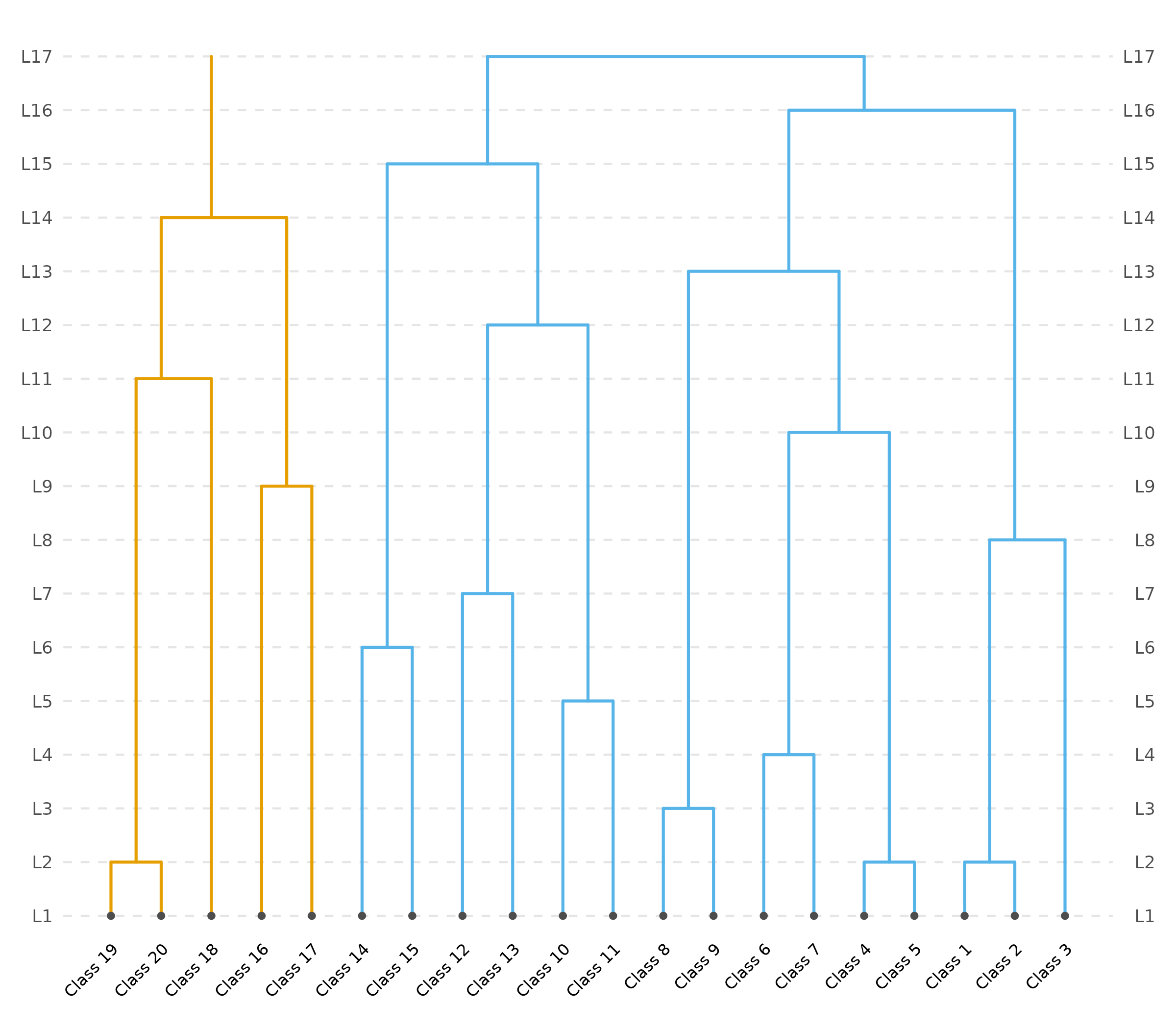
Hierarchy without choosing `segment.levels`

Unlike moneca::moneca_fast(), SBM backends return a full nested hierarchy without requiring the user to pre-specify segment.levels. The $sbm_diagnostics slot records the number of blocks and the MDL-analogue score at every level:

seg$sbm_diagnostics$n_blocks_per_level
#>  [1] 17 16 15 14 13 12 11 10  9  8  7  6  5  4  3  2
round(seg$sbm_diagnostics$mdl_per_level, 2)
#>  [1]  793.02  826.18  856.59  892.55  933.79  974.81 1019.72 1085.49 1206.58
#> [10] 1371.64 1589.59 1806.06 2027.65 2244.25 2592.20 3534.60

The adapter preserves moneca’s convention: segment.list[[1]] is atomic and segment.list[[l]] for l >= 2 runs from finest to coarsest. Passing segment.levels = 3 truncates the hierarchy to three approximately log-spaced levels while preserving the finest and coarsest.

seg3 <- moneca_sbm(mob, backend = "greed", seed = 2026, segment.levels = 3)
length(seg3$segment.list)
#> [1] 4
lengths(seg3$segment.list)
#> [1] 20  3  9  2

Empirical parity against `moneca::moneca_fast()`

If the theoretical bridge is right, moneca_sbm(backend = "greed") should recover segmentations close to those of moneca::moneca_fast() on a well-structured mobility matrix. We measure this directly with the adjusted Rand index (ARI) and normalized mutual information (NMI) between the per-node labelings produced by both methods.

ari <- function(a, b) {
  tab <- table(a, b); n <- sum(tab)
  sc <- function(x) sum(choose(x, 2))
  a_sum <- sc(rowSums(tab)); b_sum <- sc(colSums(tab))
  tab_sum <- sc(as.vector(tab))
  expected <- a_sum * b_sum / choose(n, 2)
  max_idx <- (a_sum + b_sum) / 2
  if (max_idx == expected) return(1)
  (tab_sum - expected) / (max_idx - expected)
}

nmi <- function(a, b) {
  tab <- table(a, b); n <- sum(tab); p <- tab / n
  pa <- rowSums(p); pb <- colSums(p); nz <- p > 0
  mi <- sum(p[nz] * log(p[nz] / outer(pa, pb)[nz]))
  ha <- -sum(pa[pa > 0] * log(pa[pa > 0]))
  hb <- -sum(pb[pb > 0] * log(pb[pb > 0]))
  if (ha == 0 || hb == 0) return(0)
  mi / sqrt(ha * hb)
}

level_labels <- function(mon, level) {
  n_core <- nrow(mon$mat.list[[1]]) - 1L
  labels <- rep(NA_integer_, n_core)
  cliques <- mon$segment.list[[level]]
  for (b in seq_along(cliques)) labels[cliques[[b]]] <- b
  na_idx <- is.na(labels)
  if (any(na_idx)) {
    labels[na_idx] <- max(0L, labels, na.rm = TRUE) + seq_len(sum(na_idx))
  }
  as.integer(labels)
}

fast <- moneca::moneca_fast(mob, segment.levels = 3, progress = FALSE)
sbm  <- moneca_sbm(mob, backend = "greed", seed = 2026)

fast_levels <- seq.int(2L, length(fast$segment.list))
sbm_levels  <- seq.int(2L, length(sbm$segment.list))

grid <- expand.grid(fast_lvl = fast_levels, sbm_lvl = sbm_levels)
grid$ari <- mapply(function(lf, ls) ari(level_labels(fast, lf),
                                        level_labels(sbm, ls)),
                   grid$fast_lvl, grid$sbm_lvl)
grid$nmi <- mapply(function(lf, ls) nmi(level_labels(fast, lf),
                                        level_labels(sbm, ls)),
                   grid$fast_lvl, grid$sbm_lvl)

best <- grid[which.max(grid$ari), , drop = FALSE]
best
#>    fast_lvl sbm_lvl       ari      nmi
#> 19        2       8 0.6709957 0.905422

On this 20-class synthetic fixture the best matching level pair typically recovers ARI ~ 0.67 and NMI ~ 0.90 — above the ARI >= 0.55 threshold set as the aspirational target when the direction was planned, and strong empirical confirmation of the RR ≡ DC-SBM bridge.

The match is not exact — and should not be. Clique enumeration and block-model inference are structurally different procedures: cliques insist on internal completeness at a threshold, blocks allow any stochastically-consistent edge pattern within a group. When the two agree on segmentation, the mobility data has sharply modular block structure; when they disagree, the discrepancy is itself diagnostic.

Choosing a backend

Criterion	`backend = "greed"`	`backend = "graphtool"`
Runtime install cost	`install.packages("greed")`	conda env + `graph-tool` (~800 MB)
Scale ceiling (nodes)	~10^4 – 10^5	~10^6 – 10^7
Sparse `dgCMatrix` input	yes, end-to-end	via reticulate edge list
Hierarchy construction	merge dendrogram; `cut(sol,k)`	nested MCMC, picks depth by MDL
Determinism under `seed`	high (deterministic local search)	MCMC; use `n_init` best-of-N plus `seed`
Parallel	`future` framework, portable	OpenMP; single-threaded recommended for `seed`
Portability	pure R	Python + conda

Rule of thumb: use greed until you exceed roughly 5000 nodes, then move to graphtool. The backend = "auto" default encodes this rule and falls back to greed with an informational message if graph-tool is not installed.

Installing the `graph-tool` backend

graph-tool is not distributed on PyPI, and the macOS homebrew formula compiles from source and breaks on Boost/Python version bumps. The supported route is conda-forge. moneca_sbm_install_graphtool() wraps the conda step:

monecascale::moneca_sbm_install_graphtool(envname = "moneca-sbm")
reticulate::use_condaenv("moneca-sbm", required = TRUE)

After this, moneca_sbm(backend = "graphtool") works identically to "greed". A typical install takes 2–5 minutes on a warm conda cache.

Downstream compatibility

Every moneca function that consumes a moneca object consumes a monecascale::moneca_sbm() output unchanged:

moneca::segment.membership(seg)[1:6, ]
#>      name membership
#> 1 Class 1       17.2
#> 2 Class 2       17.2
#> 3 Class 3       17.2
#> 4 Class 4       17.2
#> 5 Class 5       17.2
#> 6 Class 6       17.2

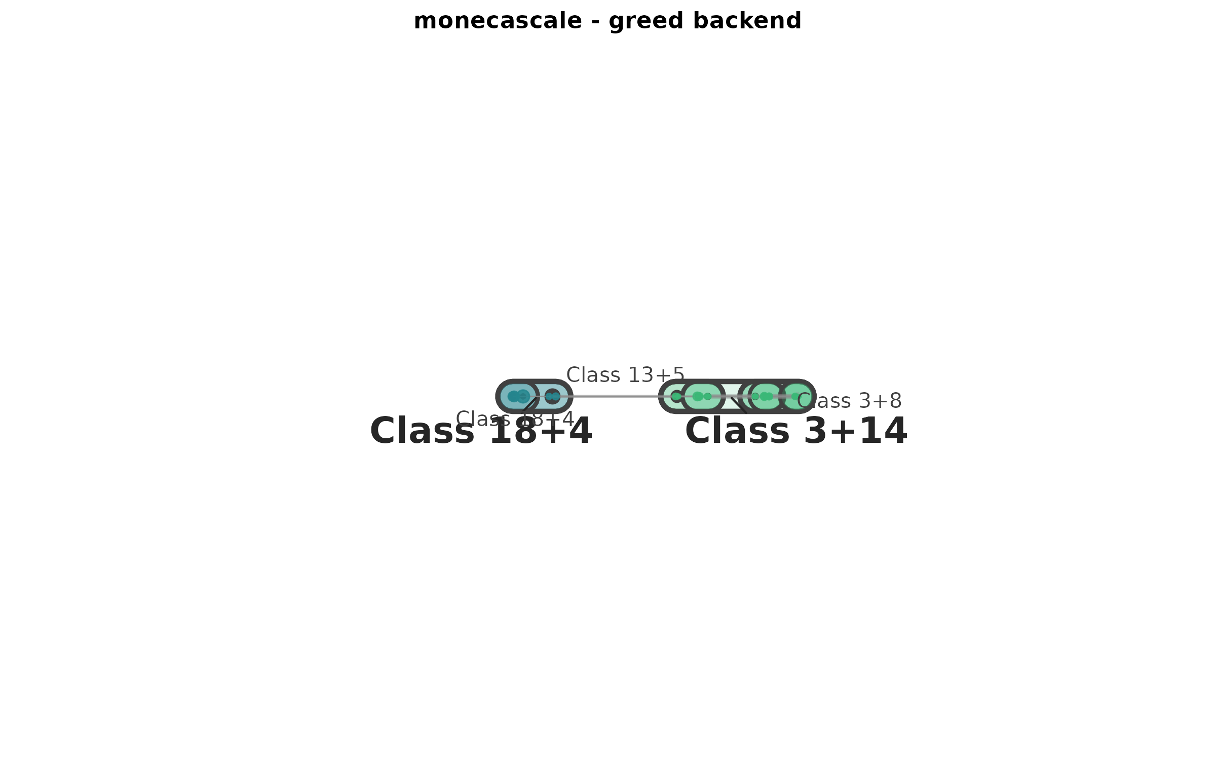
if (requireNamespace("ggraph", quietly = TRUE)) {
  moneca::plot_moneca_hierarchical(seg, title = "monecascale - greed backend")
}

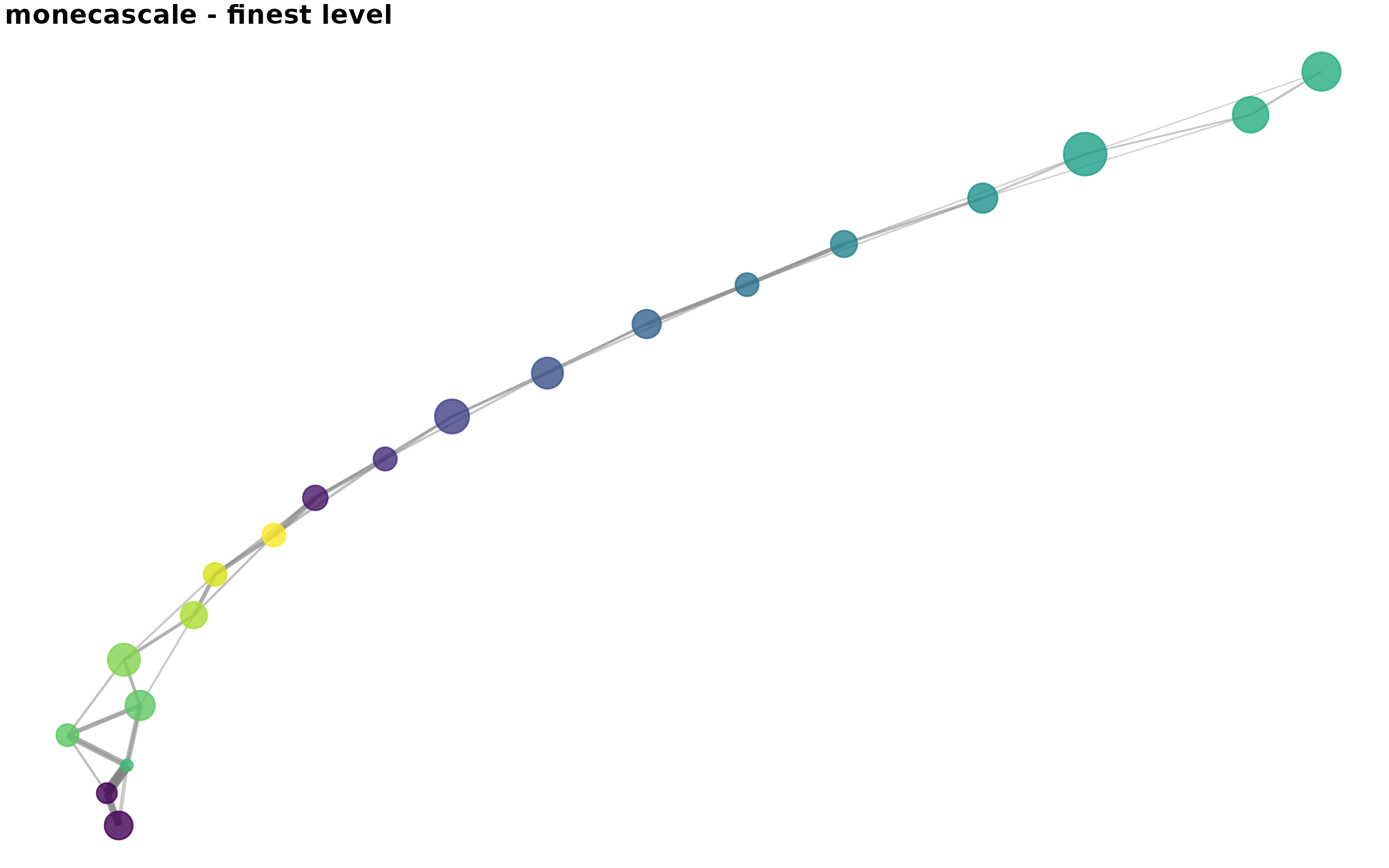
Hierarchical plot of SBM segmentation

if (requireNamespace("ggraph", quietly = TRUE)) {
  moneca::plot_moneca_ggraph(
    seg, level = 2, node_color = "segment",
    title = "monecascale - finest level"
  )
}

Network plot of finest SBM level

if (requireNamespace("ggraph", quietly = TRUE)) {
  moneca::plot_moneca_dendrogram(seg)
}

Dendrogram of SBM hierarchy

Limitations and future directions

moneca_sbm() is the first of seven directions in the MONECA scaling roadmap. Known limits on this release:

Rectangular input is not accepted. Person × employer matrices are the target use case for direction D1 (moneca_bipartite()); moneca_sbm() currently errors on non-square input with a pointer there.
Auto-level unification across backends (segment.levels = "auto" everywhere including moneca::moneca_fast()) is direction D6.
Out-of-core inference for data that does not fit in RAM is direction D7 (moneca_duckdb / moneca_arrow).

References

Karrer, B., & Newman, M. E. J. (2011). Stochastic blockmodels and community structure in networks. Physical Review E, 83, 016107.
Peixoto, T. P. (2014). Hierarchical block structures and high-resolution model selection in large networks. Physical Review X, 4, 011047.
Côme, E., & Jouvin, N. (2020). greed: Clustering and Model Selection with the Integrated Classification Likelihood. R package.
Touboel, J., & Larsen, A. G. (2017). Mapping the Social Class Structure: From Occupational Mobility to Social Class Categories Using Network Analysis. Sociology, 51(6), 1257–1276.

Giampaolo Montaletti

2026-04-24

About monecascale

The theoretical bridge: RR = O/E is the DC-SBM residual

Quick start

Hierarchy without choosing `segment.levels`

Empirical parity against `moneca::moneca_fast()`

Choosing a backend

Installing the `graph-tool` backend

Downstream compatibility

Limitations and future directions

References

monecascale: hierarchical DC-SBM backend for MONECA

Giampaolo Montaletti

2026-04-24

About monecascale

The theoretical bridge: RR = O/E is the DC-SBM residual

Quick start

Hierarchy without choosing segment.levels

Empirical parity against moneca::moneca_fast()

Choosing a backend

Installing the graph-tool backend

Downstream compatibility

Limitations and future directions

References

Hierarchy without choosing `segment.levels`

Empirical parity against `moneca::moneca_fast()`

Installing the `graph-tool` backend